Building my own language model: Transformer encoder (Part 4)

So far, we have turned raw token IDs into dense vectors that encode what a token is and where it sits in the sequence. That already feels like progress, but at this point the model still doesn’t understand anything. Each token only knows about itself.

The real work happens next: the Transformer encoder.

This is the part that lets every token look at every other token in the sequence and decide what actually matters.

Let’s look at the code first.

enc_layer = nn.TransformerEncoderLayer(
    d_model=embed_dim,
    nhead=num_heads,
    batch_first=True,
    dim_feedforward=4 * embed_dim,
    dropout=p_drop,
    activation="gelu",
    norm_first=True,
)

self.transformer = nn.TransformerEncoder(
    enc_layer,
    num_layers=num_layers
)

This may look compact, but there’s a lot hiding behind it.

One encoder layer: a repeating building block

A single Transformer encoder layer is made up of two core components:

Multi-head self-attention
Feed-forward network (MLP)

Both are wrapped with:

residual (skip) connections
layer normalization
dropout

In other words, one layer looks roughly like this:

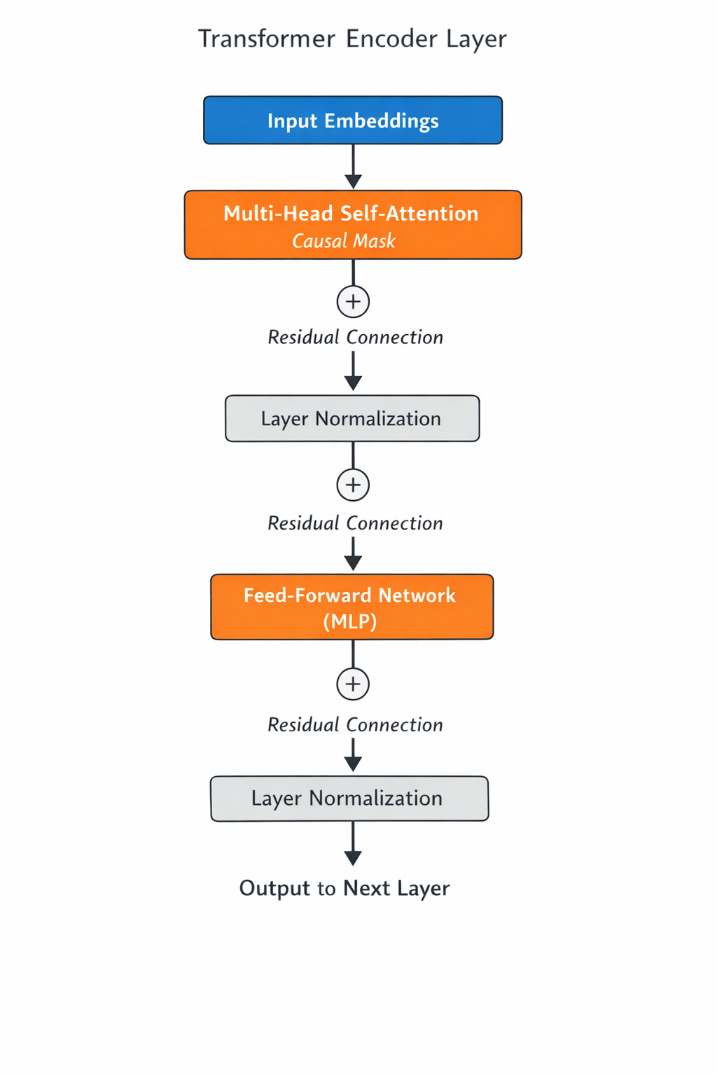
This whole block is stacked four times in our configuration, with the output of one layer feeding into the next.

Multi-head self-attention: tokens talking to each other

Self-attention is the defining idea behind transformers.

Instead of processing tokens one after another, the model processes the entire sequence at once. Each token can look at all other tokens and decide which ones are relevant to update its representation.

Internally, each token embedding is projected into three vectors:

a query
a key
a value

Attention scores are computed by comparing queries and keys, and those scores determine how values are mixed together.

The result is that each token becomes a weighted combination of other tokens in the sequence.

Why multiple heads?

In our model, attention is split into multiple heads:

NUM_HEADS = 4

Each head performs attention independently, using different learned projections.

This allows the model to capture different types of relationships at the same time. One head might focus on nearby tokens, another on longer-range dependencies, while another might pick up on structural patterns.

The outputs of all heads are then concatenated and projected back into the original embedding dimension.

Feed-forward network (MLP): thinking per token

After attention has mixed information across tokens, each token is then processed independently by a small neural network, commonly referred to as an MLP.

In the code, this is controlled by:

dim_feedforward = 4 * embed_dim

This means that for embed_dim = 128, the MLP looks like:

128 → 512 → 128

with a GELU activation in between.

This network is applied to every token separately, using the same weights.

A useful mental model is:

attention = communication between tokens
MLP = private computation per token

Residual connections and normalization

Both the attention block and the feed-forward block use residual connections, meaning their outputs are added back to their inputs.

This has two important effects:

important information is preserved
training remains stable even with many stacked layers

Layer normalization keeps activations well-scaled and prevents values from drifting into unstable ranges as depth increases.

These details may look minor, but without them, deep transformer models would be very difficult to train.

Stacking encoder layers

Finally, nn.TransformerEncoder simply stacks this layer multiple times: in our example we have 4 layers.

Each layer sees the output of the previous one and refines it further.

Early layers tend to learn more local or surface-level patterns. Later layers build increasingly abstract and contextual representations.

By the time a token exits the final encoder layer, its vector no longer represents just:

I am token X at position Y

but rather:

Given everything else in this sequence, this is what token X means here.

Why this matters

This contextualized sequence is the foundation for everything a transformer does next. For example to predict the next token: we can feed these vectors into a linear layer + softmax to produce next-token probabilities.

The encoder itself doesn’t decide what to do, it only decides what everything means.

Example

Here is a simple example, starting from an input sentence.

Sentence:

"the cat sat"

Token IDs (pretend):

the → 1
cat → 2
sat → 3

Assume:

Batch size B = 1
Sequence length T = 3
Embedding size D = 2
One attention head

1. Tokens → embeddings

Token embeddings table

the (1) → [1.0, 0.0]
cat (2) → [0.0, 1.0]
sat (3) → [1.0, 1.0]

Position embeddings

pos 0 → [0.1, 0.1]
pos 1 → [0.2, 0.2]
pos 2 → [0.3, 0.3]

Add token + position embeddings

Input to encoder:

X shape: [B, T, D] = [1, 3, 2]

X =
[
  [1.1, 0.1],   ← "the"
  [0.2, 1.2],   ← "cat"
  [1.3, 1.3]    ← "sat"
]

At this point:

tokens know who they are
tokens know where they are
tokens do not know each other

2. Self-attention (tokens processed together)

Step 2.1: create Q, K, V

For simplicity, assume:

Q = K = V = X

Step 2.2: compute attention scores

We compute:

Attention scores = Q · Kᵀ

This produces a token-to-token matrix:

shape: [T, T] = [3, 3]

Dot products:

          the     cat     sat
the   [ 1.22,   0.34,   1.56 ]
cat   [ 0.34,   1.48,   1.82 ]
sat   [ 1.56,   1.82,   3.38 ]

Each row answers:

How much should this token look at every other token?

This is the together step.

Step 2.3: softmax

After softmax, each row becomes weights that sum to 1:

the → [0.40, 0.15, 0.45]
cat → [0.10, 0.35, 0.55]
sat → [0.20, 0.25, 0.55]

Meaning for “the” → [0.40, 0.15, 0.45]

40% attention to "the"
15% attention to "cat"
45% attention to "sat"

Step 2.4: mix values (V)

Each token output is a weighted sum of all token vectors.

Example for "the":

0.40 * [1.1, 0.1] +
0.15 * [0.2, 1.2] +
0.45 * [1.3, 1.3]
=
[1.06, 0.73]

After attention, output becomes:

A =
[
  [1.06, 0.73],   ← "the" (context-aware)
  [1.05, 0.98],   ← "cat"
  [1.18, 1.09]    ← "sat"
]

MLP

Now comes the MLP. Let’s assume a tiny MLP:

2 → 4 → 2

What the MLP sees

The MLP does not see the full matrix. It sees one row at a time:

[1.06, 0.73] → MLP → [0.9, 0.2]
[1.05, 0.98] → MLP → [0.8, 0.3]
[1.18, 1.09] → MLP → [1.0, 0.4]

Output after MLP:

M =
[
  [0.9, 0.2],   ← "the"
  [0.8, 0.3],   ← "cat"
  [1.0, 0.4]    ← "sat"
]

Conclusion

The Transformer encoder is where a language model actually starts to understand context.

Embeddings give tokens identity.
Encoders give tokens relationships.

Everything that follows, prediction, sampling, and text generation, depends on the quality of these contextual representations.

In the next post we will go one step further and take a look at how the next token is not actually being predicted.