It has been a while since I had time to work on this project. Actually, the code was written a while back, but I just did not have time to write about it. Interestingly enough the initial code was co-created using GPT 4.1 and although it technically worked, the results were not great.
Therefore, while coming back to the blog, I decided to upgrade the code, using GPT 5.
Recap
I decided to build a very simple GPT model, not one that actually competes with any LLM or SLM out there, but one that helps me better understand and experience how to build a model.
- As a tokenizer I use a simple word based tokenizer
- For the tokenizer and training I use Wikitext2
- For finetuning I will use the open assist dataset, to train it on actual conversations
The crucial parts
There are a few parts needed to make this all work.
- A set of configuration parameters
- A model
- A dataset
- A training function
Configuration
I will go into more details later, but these are the configurations used at the moment.
EMBED_DIM    = 128     # size of each token/position embedding vector (hidden dimension)
NUM_HEADS    = 4       # number of attention heads per transformer layer
NUM_LAYERS   = 4       # number of stacked transformer encoder layers
SEQ_LEN      = 128     # maximum sequence length (context window)

BATCH_SIZE   = 32      # number of sequences per training batch
EPOCHS       = 1       # how many passes over the dataset to train

LR           = 3e-4    # learning rate for optimizer (step size in weight updates)
WEIGHT_DECAY = 0.01    # L2 regularization strength to prevent overfitting
GRAD_CLIP    = 1.0     # max gradient norm (prevents exploding gradients)

DROPOUT      = 0.1     # dropout probability for regularization inside the network
Model
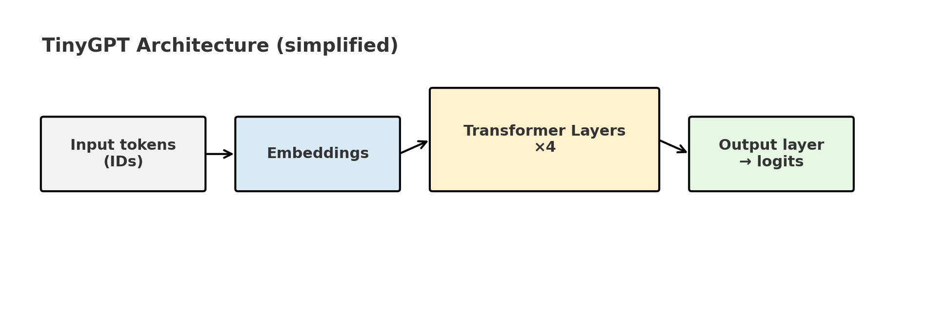
Let’s first look at the model architecture. I realized while writing the blog post that this part alone will require a few blog posts. Therefore, let’s explore the overall architecture and then dive deeper into the individual parts.
Token embeddings
Before our model can do anything clever, it has to turn our token IDs into something continuous a neural net can reason about. That’s the job of the token embedding. With a vocabulary of ~30,000 tokens and EMBED_DIM = 128, the layer is literally a table of size 30,000 × 128: one row per token, 128 numbers per row, think of “ID cards” for tokens.
# token "ID cards": one 128-D vector per vocab item
self.token_emb = nn.Embedding(vocab_size, 128)  # shape: [vocab_size, 128]
When we pass a token ID like 42, the model grabs row 42 from that table and hands you its 128-number ID card. It feels like a lookup. But during training, those numbers aren’t fixed at all, they start random and get nudged by gradient descent like any other layer. Over time, the model pushes similar words closer together (their vectors align) and pulls apart words that should behave differently. In other words, the “lookup table” is actually a learned map of meaning.
Position embeddings
Knowing who a token is isn’t enough, the model also needs to know where it is. Transformers don’t come with order built in, so we give each position its own ID card too. With SEQ_LEN = 128, that’s a second table sized 128 × 128, one row per position, each a 128-D vector.
# position "seat numbers": one 128-D vector per position in the window
self.pos_emb = nn.Embedding(128, 128)  # shape: [max_pos=128, 128]
Let’s play this through
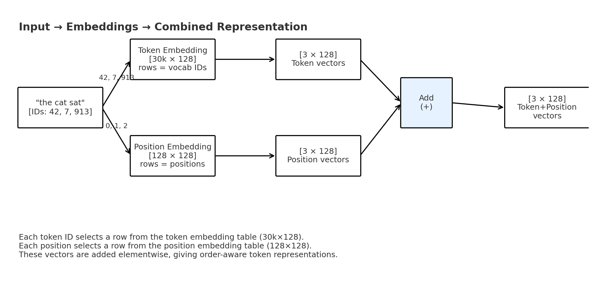
1. Raw input = token IDs
The tokenizer maps words into integers (IDs in the vocab):
"the cat sat" → [42, 7, 913]This is the raw input: just integers.
If SEQ_LEN = 128, this example sequence only uses the first 3 slots out of the available 128.
2. Token embeddings (identity)
We look these up in the token embedding table ([30,000 × 128]).
Each ID gets replaced with a 128-dimensional vector:
W_token[42]  → [128 numbers]  # "the"
W_token[7]   → [128 numbers]  # "cat"
W_token[913] → [128 numbers]  # "sat"
So now we have:
[3, 128] → 3 tokens, each with 128 features3. Position embeddings (order)
Next, we look up the position IDs: [0, 1, 2]. From the position embedding table ([128 × 128]):
pos_emb[0] → [128 numbers]  # slot 0
pos_emb[1] → [128 numbers]  # slot 1
pos_emb[2] → [128 numbers]  # slot 2
4. Combine them
We add the vectors elementwise:
"the @ pos 0" = W_token[42]  + pos_emb[0]
"cat @ pos 1" = W_token[7]   + pos_emb[1]
"sat @ pos 2" = W_token[913] + pos_emb[2]
In short
- Raw input = integers (token IDs).
- Token embedding = “who I am” (vector lookup).
- Position embedding = “where I sit” (vector lookup).
- Add them = identity + order, same size [seq_len, embed_dim].
- Feed into Transformer blocks to learn patterns and make predictions.
A quick sense of scale
- Token embedding: ~30,000 × 128 ≈ 3.8M parameters, the biggest chunk in our tiny GPT.
- Position embedding: 128 × 128 = 16,384 parameters, tiny by comparison, but important for word order.
Conclusion
Personally, I found it interesting to learn how embeddings actually work, I did realize though I had many questions. I’m not sure if the blog posts does enough justice to the complexity. But with the following blog posts everything should come together and will (hopefully) make sense.